
The unprecedented fiscal package adopted by the European Council this summer – dubbed Next Generation EU – is vital for the recovery of the euro area, write Lorenzo Codogno and Paul van den Noord. However, they estimate that the creation of a Eurobond and permanent fiscal capacity at the centre would have been a more powerful means to mitigate the impact of the crisis.
Featured Image Credit: European Council
The magnitude of the Covid-19 shock to economic activity in the Eurozone and elsewhere is unprecedented in post war history. The OECD, for instance, currently expects the Eurozone economy to shrink by 7.9% in 2020, almost twice the contraction in 2009. Yet the macroeconomic policy responses have been equally unprecedented, both at the national and pan-European levels. Most significantly, the Covid-19 pandemic finally broke the taboo on a pan-European fiscal policy, dubbed ‘Next Generation EU’.
Although the programme is not yet finalised, it is set to contain the following elements. The bulk of the fiscal expansion is provided in the form of grants and loans to member states by the Recovery and Resiliency Facility (RRF) amounting to €312.5 and €360 billion, respectively, summing up to roughly 5% of EU GDP. While the exact formulas are still under discussion, the intention is to spread out the transfers over the years 2021 to 2025, with the onus of the support on those countries that have been hit the most by the crisis. Alongside the RRF, member states would receive €77.5 billion under a range of other programmes, such as ‘ReactEU’ and the Just Transition Fund.
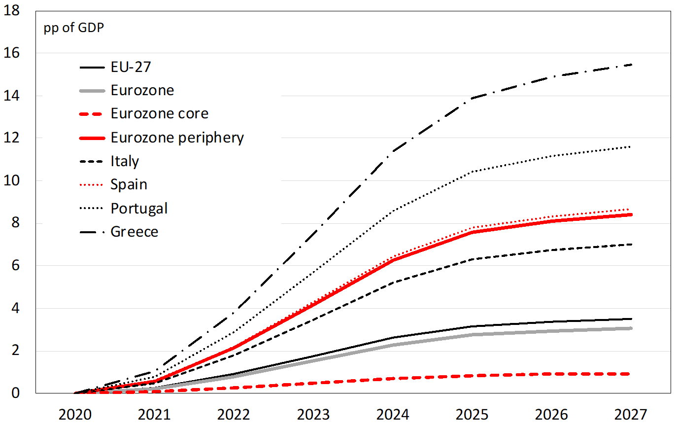
Using conservative assumptions on the multiplier effects, we estimate the impact on Eurozone economic growth to be a cumulative 1.5% by 2023 and 3.0% by 2027 (Figure 1). Most of this will benefit the Eurozone periphery, where the cumulative effect could be as large as 4% by 2023 and well over 8% in 2027.1 While impressive enough, this is excluding the impact of a range of other – national and supranational – policy initiatives that need to be taken into consideration as well. This will tell us whether or not Next Generation EU is indeed the game-changer it is intended to be, or not.
We use a stylised macroeconomic model developed in a recent paper that is aimed at capturing the cumulative impact of policy change over the medium run. We proceed in two steps, broadly reflecting the chronology of events. First, we look at both the national and pan-European fiscal responses (e.g. SURE) which were primarily shaped during the initial stages of the outbreak and the associated lockdowns in the spring, as well as the ECB’s monetary policy response. Next, we add in the impact of Next Generation EU.
Figure 1: Next Generation EU – estimated cumulative impact on real GDP
Source: European Commission, European Council, authors’ own calculations.
Finally, we compare these policy responses to a hypothetical case in which an alternative macroeconomic policy and governance framework is assumed along the lines of our paper. Specifically, we assume (i) a single Eurobond to replace national bonds on banks’ balance sheets so as to break the link between banking and sovereign distress, (ii) Eurozone fiscal capacity, including automatic stabilisers and discretionary (but rules-based) policy, and (iii) a new quantitative easing (QE) scheme that mandates the ECB to purchase Eurobonds (while national sovereigns lose QE eligibility and those still on the ECB’s balance sheet are swapped for Eurobonds as well).
All simulations assume that the core and the periphery are hit by an adverse demand shock of respectively -10% and -15% of GDP and an adverse supply shock of respectively -5% and -7.5% of GDP. This is obviously a very crude gauge of the Covid-19 shock, and views are bound to evolve as information flows in. Also, we assume a favourable risk premium shock of -200 bps in the core – and hence an equivalent shock to the spread – due to a flight to safety (this is aside from the endogenous change in the spread in response to the changes in debt positions).
Actual policy
Table 1 reports the computed changes in main aggregates and policy variables in the core, periphery and euro area at large. The first column, labelled ‘I’, shows the combined impact of:
1. Monetary policy stimulus consisting of a sustained 25bp cut in the policy rate2 and asset purchases amounting to 12.3% of GDP per annum sustained for two years.3 We also assume an exogenous cut in the periphery yield by 200 bps over and above the impact of the ECB’s asset purchases to reflect the availability of a new ESM credit line (though this may never be used for various reasons).
2. Fiscal stimulus amounting to 5.2% of GDP in the core and 3.2% of GDP in the periphery.4 Besides, we factor in a range of pan-EU measures adopted in the spring, such as React EU, that involve fiscal stimulus of the order 0.4% of GDP in the core and 0.8% in the periphery.
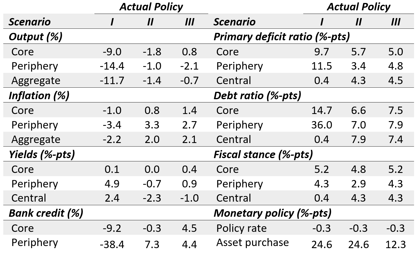
Table 1: Shock-responses
Note: Scenarios refer to: I = National fiscal responses + SURE + ESM credit line + monetary policy, II = I + ‘Next Generation EU’, III = Safe asset + permanent fiscal capacity.
Column II of the table reports the computed outcomes of the actual policy, including the impact of Next Generation EU. Specifically, while leaving all other assumptions unchanged, it is assumed additionally that:
1. Grants are allocated under the Recovery and Resilience Facility to the tune of 1.0% of local GDP in the core and 4.5% of local GDP in the periphery. As a result, the increase in the primary deficit at the centre would average around 3.5% of euro area GDP.
2. Loans are allocated to the tune of 0.4% of local GDP in the core and 6.7% of local GDP in the periphery. This leaves the primary deficit at the centre unaffected (loans are below the line). Still, it does have an impact on EU-debt (and a corresponding issuance of common bonds) of an additional 3.5% of Eurozone GDP.
3. About 20% of the above Next Generation EU package is assumed to be used for funding of existing national measures, which therefore would reduce the national fiscal stimulus accordingly.
The main results of the simulation can be summarised as follows:
1. The contraction of output is considerably smaller (-1.5%) with much less divergence between the core and periphery. The widening yield spread would be neutralised as well, while bank credit would not shrink. So, the package would be quite effective according to our stylised model.
2. On the fiscal side, we see the primary deficits at the national level still increasing substantially by 6% of GDP in the core and 3.5% of GDP in the periphery. Yet, especially in the periphery, this is a much smaller increase than in scenario I, helped by the more favourable macroeconomic environment, the less prevalent automatic fiscal stabilisers and the use of transfers from the centre to fund national programmes. The same holds for the public debt position.
Policy response with a safe asset and fiscal capacity
Scenario III reported in Table 1 is based on the following assumptions:
1. We maintain all national policy measures as well as the creation of the ESM credit line as assumed in scenarios I and II. We also assume the supranational fiscal stimulus (both loans and grants) on aggregate to be the same as in scenario II, but instead with the fiscal stimulus used to fund pan-European (as opposed to national) programmes and projects. The rationale for this choice is to avoid the crowding out of national spending programmes. We also slash the asset purchases by the ECB by half.
2. Alongside discretionary fiscal expansion at the centre, we assume supranational automatic fiscal stabilisers to cater for some horizontal redistribution. This could be the result of a centralised unemployment insurance or re-insurance scheme or the creation of a rules-based European buffer fund, for example. Specifically, we assume that for every 1 percentage point contraction in national GDP, an automatic transfer of 0.2 percentage points of national GDP would occur. This transfer replaces equivalent national automatic stabilisers to provide genuine fiscal relief.
3. We assume that a safe asset (the same common bond that is issued to raise money for fiscal stimulus at the centre) is created before the pandemic and swapped for national sovereigns on banks’ balance sheets to remove the bank-sovereign doom loop. We also assume that only the safe asset has been made eligible for purchases by the ECB. Hence all asset purchases carried out by the ECB in this scenario refer to purchases of the safe asset (in the secondary market).
The main results can be summarised as follows:
1. The aggregate stabilisation is more potent than in scenario II, though this is entirely attributable to the stabilisation of output in the core. This is not surprising given the absence of (discretionary) fiscal transfers. Yet the periphery is not (much) worse off relative to scenario II. Even so, the yield spread widens somewhat relative to scenario II, reflecting the absence of sovereign debt purchases by the ECB, but without affecting bank lending as the doom loop is broken.
2. The fiscal-monetary policy mix has shifted towards the former, with the aggregate fiscal deficit at the centre widening more than in scenario II – as the supranational automatic stabilisers kick in – and the asset purchases halved. Since the ECB would purchase the common bond only, its yield is now disconnected from the national yields and falls relative to them.
All in all, with a safe asset and a (partly rules-based) fiscal capacity, more of the pandemic shock would have been absorbed, with less quantitative easing needed. Moreover, the asset purchases would be directed to the safe asset rather than national sovereigns and hence avoid the political conflict this could entail and the need to keep the purchases in check with the capital key. The current policy response could be seen as a second-best, i.e. a less efficient way to respond to an economic shock, although still powerful, if not vital. This exercise shows that it would be worthwhile considering a more permanent macroeconomic stabilisation mechanism in the future.
Notes
1. The ‘core’ includes Belgium, Germany, France, Netherlands, Austria, Finland, Luxembourg, and, for the purpose of this exercise also Estonia and Ireland. All other Eurozone countries are included in the periphery.
2. This refers to the PELTROs which are available at a rate 25 bps below the REFI of -0.5%.
3. This comprises the additional envelope of the Asset Purchase Programme (APP) of €120 billion adopted in March 2020 and the Pandemic Emergency Purchase Programme (PEPP) with an envelope of €1,350 billion adopted in June 2020 (including an initial envelope of €750 billion adopted in March). Both are assumed to be extended by another year to a total of €2,940 billion or 24.6% of 2019 GDP.
4. Estimates based on data from Bruegel with some modifications.